In 2017 the University of California launched Career Tracks, a job classification system for staff not represented by a union. The goal was threefold: (1) to give employees better-defined career paths; (2) to better-align university compensation with the market; and (3) to better-reflect primary job responsibilities for each employee. Additionally, Career Tracks is meant to promote greater transparency in hiring and promotions. Employees can now chart their UC careers via a hierarchy of job families and functions, each with specified education levels, scopes, and responsibilities. And while the initial feedback has been positive, the overall success of the program remains to be seen.
Career Tracks is meant to create a coherent bureaucracy. I don’t mean that pejoratively. Rather, Career Tracks expresses an institutional dichotomy–these individuals perform these tasks, these individuals perform other tasks, and so on and so forth. It is the important work of a massive, complex economy of peoples, benefitting individuals at every level. It is human resources writ large.
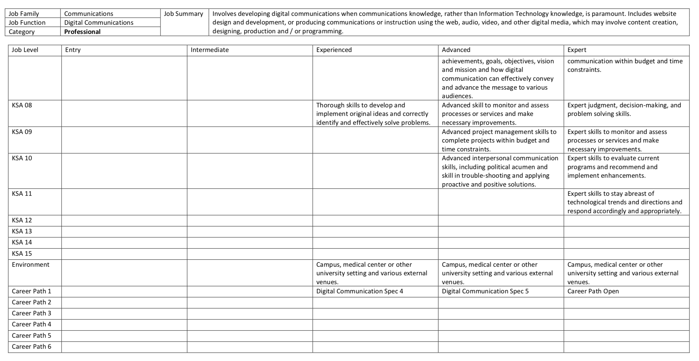
Career Tracks is instantiated by hundreds of job templates and tables. These tables communicate almost everything you need to know about every UC position. They are concise, precise, and well-written. But unfortunately, the information is squirreled away in hideous tables within .pdf and .docx files. There is subtle irony here: while Career Tracks makes grand claims to transparency, the vehicles of its standards are barely human or machine readable. Here is what the Digital Communications job template looks like:
You may have guessed where this is going. The language of Career Tracks almost cries out for text mining, and the general hideousness of the templates demand cleaning and tidying. Tasks for which both R and my blog are particularly well-suited. In Part I I’ll work through the cleaning process, and in Part II I’ll venture a sentiment analysis of UC bureacracy.
My code for the cleaning process is below. I leaned heavily on the tabulizer and docxtractor packages,
but the former did a poor job parsing the tables within each files. As you can see in the visdat below,
I was only able to parse about 20% of the templates, a disappointing number. Fortunately, I was able to obtain the salary grades
and other information from other sources.
I begin by loading the required libraries, unzipping the files, and defining some preliminary functions that would prove useful later:
library(tidyverse)
library(tabulizer)
library(docxtractr)

unzip("Career Tracks Templates.zip")
files <- dir("Career Tracks Templates", full.names = TRUE)

set_row_as_names <- function(x, row_num, clean = TRUE) {
  new_header <- as.vector(unlist(x[row_num,]))
  x <- x[-c(1:row_num),]
  names(x) <- new_header
  if (clean) return(janitor::clean_names(x))
  x
}

transpose_as_tibble <- function(x) as_tibble(t(x))

unite_common_columns <- function(x) {
  unite_s <- partial(unite, sep = " ")
  x <- janitor::clean_names(x)
  if ("licensure_1" %in% names(x)) x <- rename(x, license_1 = licensure_1)
  x %>% unite_s(key_responsibilities, key_resp_01:key_resp_15) %>%
    unite_s(education, education_1:education_4) %>%
    unite_s(ksa, ksa_01:ksa_15) %>%
    unite_s(certifications, cert_1:cert_4) %>%
    unite_s(special_conditions, spec_cond_1:spec_cond_4) %>%
    unite_s(licenses, license_1:license_4) %>%
    unite(career_path, career_path_1:career_path_6, sep = ", ") %>%
    mutate_all(funs(stringr::str_remove_all(., "NA"))) %>%
    mutate_all(funs(stringr::str_trim(.))) %>%
    naniar::replace_with_na_all(~.x == "")
}

coerce_numeric <- function(x) {
  s <- gsub(",", "", x)
  as.numeric(s)
}
Then I defined two additional functions, one to parse PDFs and another to parse .docx files. Why the templates are stored with alternating file extensions is beyond me.
parse_pdf_tables <- function(pdf_file) {

  all_tables <- tabulizer::extract_tables(pdf_file)

  ### If tabulizer fails to parse tables and only returns headers
  if (all(dim(all_tables[[2]]) == c(3,4))) return(NULL)

  table_ind <- seq(0, length(all_tables) + 1, 2)[-1]
  job_table <- all_tables[table_ind] %>%
    discard(is.null) %>%
    map(as_tibble) %>%
    map(naniar::replace_with_na_if,
        .predicate = is.character,
        condition = ~.x == "") %>%
    map(fill, V1) %>%
    map_df(fill, V1)

  meta <- transpose_as_tibble(job_table[c(1:6),])) %>% set_row_as_names(1)

  job_table <- job_table[-c(1:6),]
  job_table %>%
    filter(V1 != "Job Level") %>%
    group_by(V1) %>%
    summarize_all(funs(paste(., collapse = " "))) %>%
    ungroup() %>%
    transpose_as_tibble() %>%
    set_row_as_names(1) %>%
    unite_common_columns() %>%
    bind_cols(meta) %>%
    janitor::clean_names()
}

parse_docx_tables <- function(docx_file) {

  docx <- docxtractr::read_docx(docx_file)
  suppressMessages(docxtractr::docx_extract_all_tbls(docx, guess_header = FALSE))[[1]] %>%
    transpose_as_tibble() %>%
    set_row_as_names(1) %>%
    unite_common_columns()
}
Some highlights: the nanair and janitor packages, as well as fill() from the tidyr package. Transposing the entire
table was also a nifty trick.
For extra trick points, I created a progress bar while mapping over the entire directory of files:
parse_file_tables <- function(x, .pb = NULL) {
  .pb$tick()$print()
  if (grepl(".docx$", x)) return(parse_docx_tables(x))
  if (grepl(".pdf$", x)) return(parse_pdf_tables(x))
}

pb <- progress_estimated(length(files))
safe_parse <- safely(parse_file_tables)
career_tracks_list <- map(files, safe_parse, .pb = pb)

career_tracks <- career_tracks_list %>%
  discard(is.null) %>%
  map_df("result") %>%
  select(contains("job"), everything())
  mutate(per_program = coalesce(per_program, personnel_program)) %>%
  select(-job_level1, -job_level2, -job_level3, -key_resp_01, -key_resp_011, -personnel_program)
As there were over 300 templates, this operation took several minutes, but it was cool to see the countdown. I was able to speed things up a little by postponing some additional formatting until I had one large table instead of reshaping hundreds of little tables and then joining them together. A visual sequence of the cleaning and tidying sequence in the gif below, courtesy of ViewPipeSteps:
Finally, I downloaded some additional files and joined them all together:
download.file("http://shr.ucsc.edu/policy/special-projects/career-tracks/Resources/Career%20Tracks%20Job%20Title%20Listing%202-15-17.pdf",
              destfile = "career_tracks_info.pdf")
download.file("http://shr.ucsc.edu/policy/special-projects/career-tracks/Resources/Salary%20Range%20Structure_July2016.pdf",
              destfile = "career_salary_grades.pdf")

career_tracks_info <- tabulizer::extract_tables("./career_tracks_info.pdf")
salaries <- tabulizer::extract_tables("./career_salary_grades.pdf")

career_tracks_info <- career_tracks_info %>%
  map_df(data.frame) %>%
  set_row_as_names(1)

salaries <- salaries %>%
  map_df(data.frame) %>%
  set_row_as_names(2)

career_tracks <- career_tracks %>%
  left_join(career_tracks_info %>%
              filter(job_family != "Job Family") %>%
              select(job_family:job_code, status, grade), by = "job_code") %>%
  left_join(salaries, by = "grade") %>%
  mutate_at(vars(matches("grade|minimum|midpoint|maximum")), coerce_numeric) %>%
  select(contains("job"), everything())
Here’s a View() of the data now:
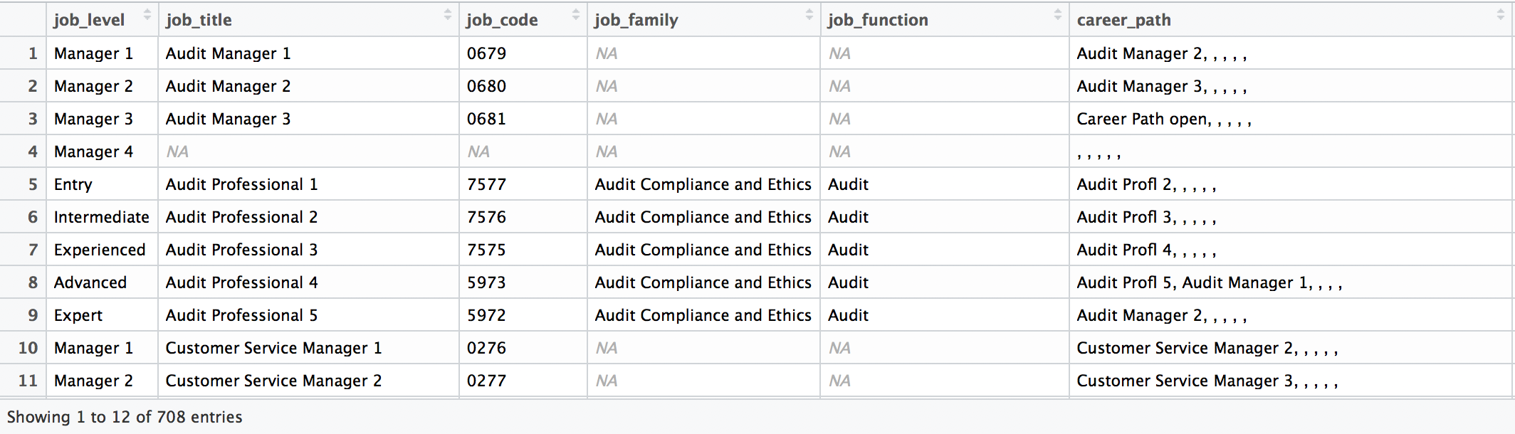
Better. But I admit the final vis_miss was disappointing:
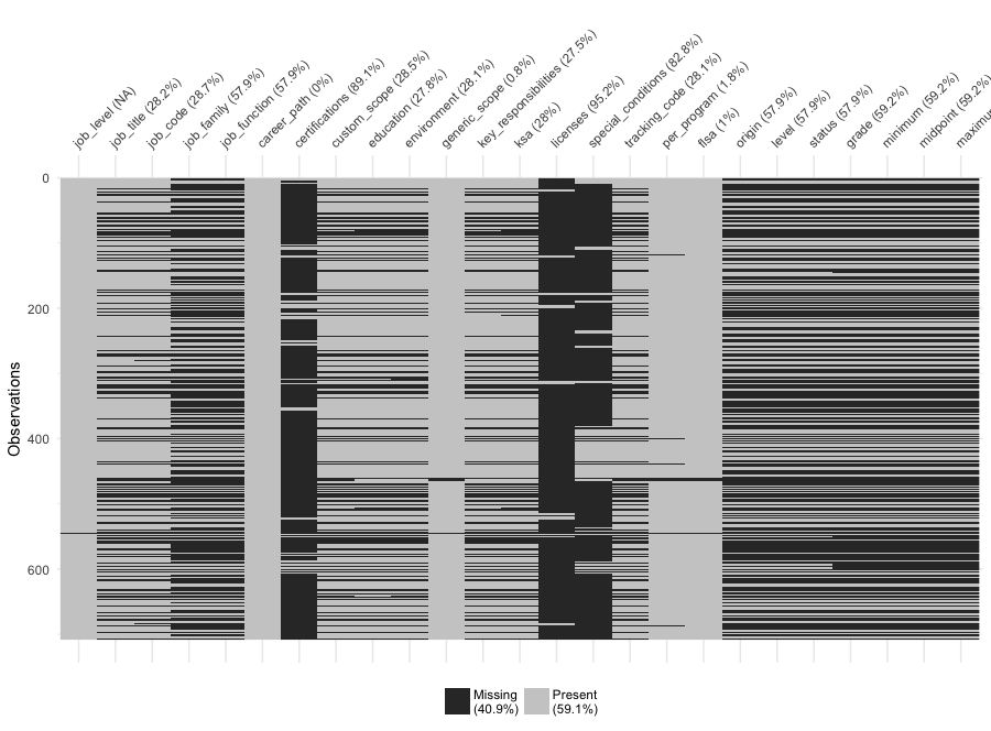
Whether this is a healthy sample remains to be seen in Part II. In the meantime, I may ponder how to get more of the missing data…