I have yet to learn the tidy evaluation paradigm. Typically, violating DRY principles with a combination of hacks and brute force gets the job done. But a recent challenge at work took me perilously to the edge.
The task was this: calculate the ratio of returning and new students by academic quarter. Our working definition of a returning student is having taken any course in a previous quarter.
Let’s build some sample data:
library(tidyverse)

set.seed(2018)

ids <- 1:5000
start_dates <- seq(as.Date("2010/01/01"), as.Date("2018/05/18"), by = "day")
departments <- c("Math", "Science", "English", "History", "Modern Languages")

generate_data <- function(reps, samp, size) {
  c(replicate(size, sample(samp, size = size, replace = TRUE)))
}

ids <- generate_data(100, ids, 100)
departments <- generate_data(100, departments, 100)
start_dates <- start_dates %>%
  sample(500, TRUE) %>%
  sample(10000, TRUE)

df <- tibble(
  student_id = ids,
  department = departments,
  class_start_date = start_dates
) %>%
  mutate(quarter = lubridate::quarter(class_start_date),
         year = lubridate::year(class_start_date)) %>%
  mutate(
    quarter = case_when(
      quarter == 1 ~ "Winter",
      quarter == 2 ~ "Spring",
      quarter == 3 ~ "Summer",
      quarter == 4 ~ "Fall"
      ),
    school = case_when(
      department %in% c("Math", "Science") ~ "STEM",
      TRUE ~ "Liberal Arts"
      )
    ) %>%
  mutate(quarter = paste(quarter, year)) %>%
  select(student_id, school, department, class_start_date, quarter, year)
A glace at our generated data:
# A tibble: 10,000 x 6
   student_id school       department       class_start_date quarter      year
        <int> <chr>        <chr>            <date>           <fct>       <dbl>
 1       1681 Liberal Arts History          2010-03-14       Winter 2010 2010.
 2       2319 STEM         Math             2013-03-29       Winter 2013 2013.
 3        303 Liberal Arts English          2014-08-04       Summer 2014 2014.
 4        988 STEM         Science          2011-07-14       Summer 2011 2011.
 5       2372 Liberal Arts English          2013-11-26       Fall 2013   2013.
 6       1506 Liberal Arts English          2012-01-11       Winter 2012 2012.
 7       3034 STEM         Math             2017-10-24       Fall 2017   2017.
 8        651 Liberal Arts English          2013-11-03       Fall 2013   2013.
 9       4794 Liberal Arts Modern Languages 2015-02-08       Winter 2015 2015.
10       2735 STEM         Science          2012-03-24       Winter 2012 2012.
# ... with 9,990 more rows
To calculate the ratios, I had to encode the quarter variable as a factor. And to get the chronological levels, I arranged the data frame by class start date, pulled out the unique quarters, and factored the original quarter variable with the appropriate levels.
quarters <- df %>%
  arrange(class_start_date) %>%
  pull(quarter) %>%
  unique()
quarters <- factor(quarters, levels = quarters)

df <- df %>% mutate(quarter = factor(quarter, levels = quarters))
A useful attribute of factors is that they can be converted to integers. For example, note how each factor level corresponds to an ascending integer:
> quarters
 [1] Winter 2010 Spring 2010 Summer 2010 Fall 2010   Winter 2011 Spring 2011 Summer 2011 Fall 2011
 [9] Winter 2012 Spring 2012 Summer 2012 Fall 2012   Winter 2013 Spring 2013 Summer 2013 Fall 2013
[17] Winter 2014 Spring 2014 Summer 2014 Fall 2014   Winter 2015 Spring 2015 Summer 2015 Fall 2015
[25] Winter 2016 Spring 2016 Summer 2016 Fall 2016   Winter 2017 Spring 2017 Summer 2017 Fall 2017
[33] Winter 2018 Spring 2018
34 Levels: Winter 2010 Spring 2010 Summer 2010 Fall 2010 Winter 2011 Spring 2011 ... Spring 2018

> as.integer(quarters)
 [1]  1  2  3  4  5  6  7  8  9 10 11 12 13 14 15 16 17 18 19 20 21 22 23 24 25 26 27 28 29 30 31 32 33
[34] 34
I then tried to imagine the data frame as a timeline with the temporal markers as quarters. For example, I could identify all the new students for a given quarter by (1) subsetting the data with all quarters “less than” (earlier than) that specific quarter, (2) identifying the unique quarters by student, and (3) filtering for the quarter, and then checking if the unique quarters match the given quarter.
The entirety of my function is below, but I’ll break the pipeline down here.
Step 1: Filtering all Earlier Quarters
The quarter_td argument is first factored with the same levels as the data frame, then converted to an integer. I’m then able to filter the earlier quarters within the data frame.
calc_new_students <- function(quarter_td, ...) {

  quarter_td_int <- as.integer(factor(quarter_td, levels = quarters))

  df %>%
    filter(as.integer(quarter) <= quarter_td_int)
    ...
}
  calc_new_students("Fall 2015", department) %>%
    distinct(quarter) %>%
    arrange(desc(quarter))
# A tibble: 24 x 1
   quarter
   <fct>
 1 Fall 2015
 2 Summer 2015
 3 Spring 2015
 4 Winter 2015
 5 Fall 2014
 6 Summer 2014
 7 Spring 2014
 8 Winter 2014
 9 Fall 2013
10 Summer 2013
# ... with 14 more rows
Step 2: Indentify Unique Quarters by Student
Collapsing the unique quarters into a vector produces a snapshot of their registration history.
calc_new_students <- function(quarter_td, ...) {

    ...
    group_by(student_id) %>%
    mutate(unique_quarters = paste(unique(quarter), collapse = ", ")) %>%
    ungroup()
    ...
}

calc_new_students("Fall 2015") %>%
  select(student_id, unique_quarters)
# A tibble: 7,083 x 2
student_id unique_quarters
<int> <chr>
1 1681 Winter 2010, Winter 2012
2 2319 Winter 2013, Summer 2013, Winter 2012, Fall 2010
3 303 Summer 2014, Summer 2010
4 988 Summer 2011, Spring 2012, Fall 2011, Spring 2013
5 2372 Fall 2013, Winter 2012, Winter 2015
6 1506 Winter 2012, Winter 2010, Fall 2012
7 651 Fall 2013, Winter 2010, Summer 2012, Fall 2012, Summer 2015
8 4794 Winter 2015
9 2735 Winter 2012, Spring 2014, Winter 2011, Fall 2013
10 4911 Spring 2012, Fall 2013
# ... with 7,073 more rows
Step 3: Indentify New and Returning Students
If a student’s unique_quarters is length one and matches the quarter argument, they are a new student. If not, they are a returning student.
calc_new_students <- function(quarter_td, ...) {

    ...
    filter(as.integer(quarter) == quarter_td_int) %>%
    distinct(student_id, .keep_all = TRUE) %>%
    mutate(student = if_else(unique_quarters == quarter_td, "New", "Returning"))
    ...
}

calc_new_students("Fall 2015") %>%
  select(student_id, student)
# A tibble: 350 x 2
student_id student
<int> <chr>
1 1301 New
2 3022 New
3 2049 Returning
4 3229 Returning
5 1610 Returning
6 2671 Returning
7 3857 New
8 431 New
9 2383 Returning
10 1311 Returning
# ... with 340 more rows
Step 4: Group the New and Returning Students by Other Columns
I’m able to generalize the function to group by other column names by passing them through ....
calc_new_students <- function(quarter_td, ...) {

    ...
    group_by(student, ...) %>%
    summarize(students = n()) %>%
    arrange(...) %>%
    mutate(quarter = quarter_td)
}

calc_new_students("Fall 2015", department)
calc_new_students("Fall 2015", school)
# A tibble: 10 x 4
# Groups: student [2]
student department students quarter
<chr> <chr> <int> <chr>
1 New English 15 Fall 2015
2 Returning English 62 Fall 2015
3 New History 15 Fall 2015
4 Returning History 54 Fall 2015
5 New Math 14 Fall 2015
6 Returning Math 65 Fall 2015
7 New Modern Languages 17 Fall 2015
8 Returning Modern Languages 45 Fall 2015
9 New Science 23 Fall 2015
10 Returning Science 40 Fall 2015
# A tibble: 4 x 4
# Groups:   student [2]
  student   school       students quarter
  <chr>     <chr>           <int> <chr>
1 New       Liberal Arts       47 Fall 2015
2 Returning Liberal Arts      161 Fall 2015
3 New       STEM               37 Fall 2015
4 Returning STEM              105 Fall 2015
Here’s a sequence of the transformations, courtesy of ViewPipeSteps:
Step 5: Iterate through all Quarters
Now we can loop through all the quarters and bind the new and returning students into a data frame:
all_quarters <- quarters %>%
  map_dfr(calc_new_students)
And a final visualization!
ggplot(all_quarters, aes(quarter, students, fill = student)) +
  geom_bar(stat = "identity", position = "fill") +
  geom_hline(yintercept = 0.5, linetype = "dashed") +
  labs(x = "Quarter",
       y = "",
       title = "Ratio of New and Returning Students",
       subtitle = "2010-2018") +
  hrbrthemes::theme_ipsum() +
  theme(axis.text.x = element_text(angle = 45))
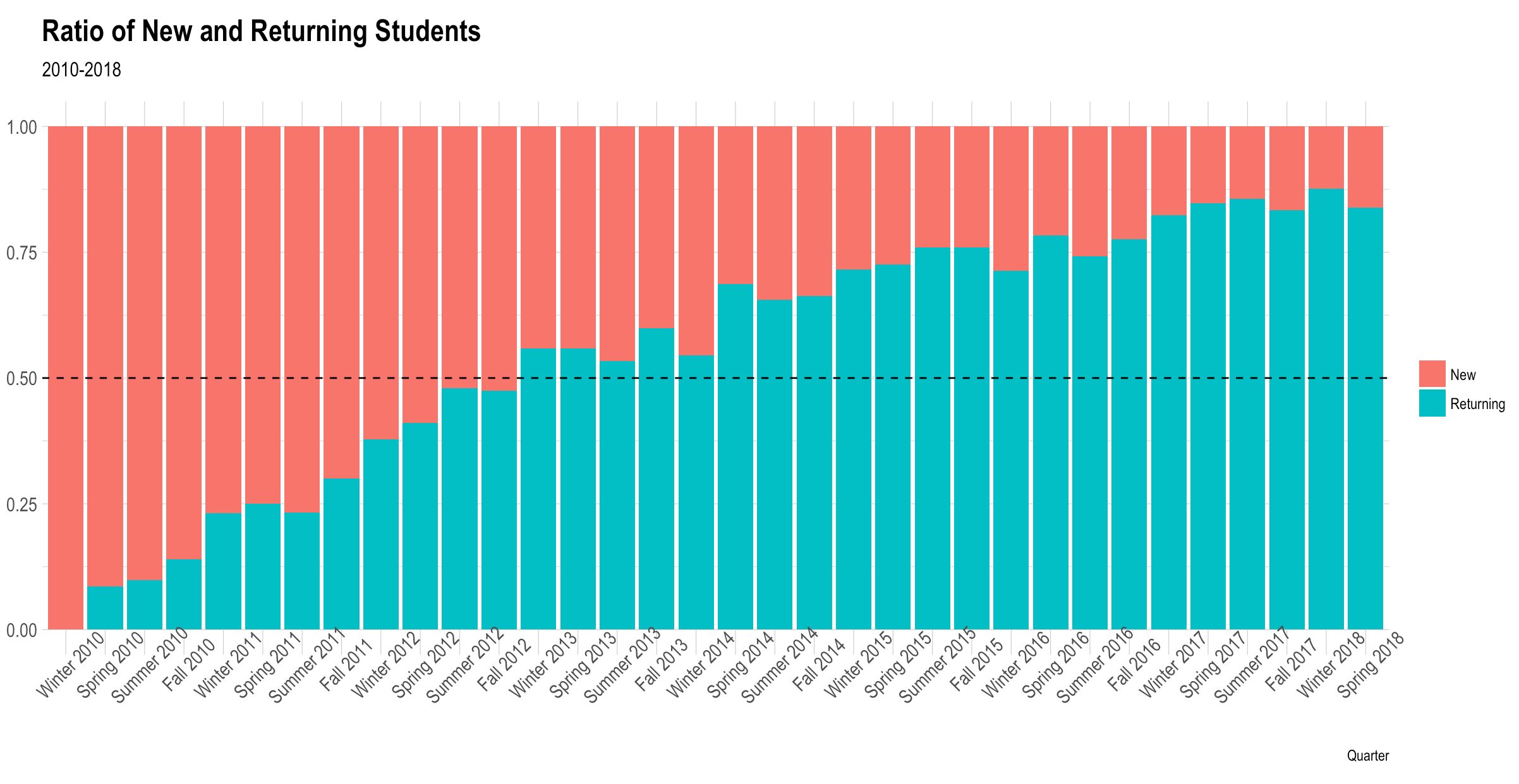 Obviously in this closed, generated data, the proportion of returning students grows with each successive quarter. But with
some additional tinkering, some interesting, seasonal, patterns may emerge.
Obviously in this closed, generated data, the proportion of returning students grows with each successive quarter. But with
some additional tinkering, some interesting, seasonal, patterns may emerge.